Distributome Colorblindness Activity

Overview

Colorblindness – Can you see the number in this image? 

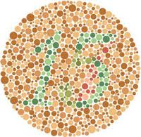
This Distributome Activity illustrates an application of probability theory to study Colorblindness, typically a genetic disorder which results from an abnormality on the X chromosome. The condition is thus rarer in women since a woman would need to have the abnormality on both of her X chromosomes in order to be colorblind (whether a woman has the abnormality on one X chromosome is essentially independent of having it on the other).

Goals

The goal of this activity is to demonstrate an efficient protocol of estimating the probability that a randomly chosen individual may be colorblind.

Hands-on Activity

Suppose that \(p\) is the probability that a randomly selected ”man” is colorblind.

• 100 men are selected at random. What is the distribution of \(X_m\) = the number of these men that are colorblind?

Answer
\(X_m\) ~ \(Binomial(100,p)\)

• 100 women are selected at random. What is the distribution of \(X_f\) = the number of these women that are colorblind?

See Hint
The chance that an individual woman is colorblind is \(p^2\), why?

Answer
\(X_f\)~\(Binomial(100,p^2)\)

• To estimate the probability that a randomly selected woman is colorblind, you might use the proportion of colorblind women in a sample of n women. What is the variance of this estimator?

Answer
\(X_f\)~\(Binomial(n,p^2)\).
Thus \(Var(\frac{X_f}{n}) \equiv \frac{p^2(1-p^2)}{n}\).

• Alternatively, to estimate the probability that a randomly selected woman is colorblind, you might use the square of the proportion of colorblind men in a sample of n men. Explain why this estimate makes sense. What is the variance of this estimator?

  See Hint
  The moment generating function can be used to find the fourth moment about the origin.

  Answer
  We want to estimate \(p^2\) and \(\frac{X_m}{n}\) estimates \(p\) so it makes sense to use \((\frac{X_m}{n})^2\) as the estimator (in fact it will be the maximum likelihood estimate. We have \(Var[( \frac{X_m}{n} )^2 ] \equiv n^{-4}[E(X_m^4 ) – (E(X_m^2 ))^2 ]\). Take \(q \equiv 1-p\). Then the fourth moment about the origin of a binomial is \(E(X^4) \equiv np(q-6pq^2+7npq-11np^2q+6n^2p^2q+n^3p^3)\) and the second moment is \(E(X^2) \equiv np(q+np)\). Thus \(Var[( \frac{X_m}{n} )^2 ] \equiv n^{-3}(pq + 6(n-1)p^2q^2 + 4n(n-1)p^3q)\).
  

• For large samples, is it better to use a sample of men or a sample of women to estimate the probability that a randomly selected women is colorblind? Explain.

See Hint
Show that a normal approximation is valid for both and then compare the variances.

Answer
For large n the ratio of the variances for the estimate in part c to the estimate in part d is \(\frac{Var(\frac{X_f}{n})}{Var((\frac{X_m}{n})^2 )} \sim \frac{p^2(1-p^2)}{4p^3q} \equiv \frac{1+ p}{4p}\). When this ratio is greater than 1, the estimator based on the sample of men will be better. Since this happens for any \(p < \frac{1}{3}\), which is clearly the case for colorblindness, it is better to use a sample of men to estimate the probability that a random woman is colorblind.

Alternate approach

You can also use the delta method to find the approximate variance for the estimator above.

Conclusions
In practice, it may difficult to obtain reliable parameter estimates when the event at hand is very rare (such as with colorblindness in women). The use of a valid probability model such as the relationship between the chance of colorblindness in men and the chance in women may improve these estimates.

Distributome Homicide Trends Activity

Overview

A Columbus Dispatch newspaper story on Friday January 1, 2010 discussed a drop in the number of homicides in the city the previous year. Here are the first few paragraphs from the article:

• Homicides take big drop in city: Trend also being seen nationally, but why is a mystery.
• The number of homicides in Columbus dropped 25 percent last year after spiking in 2008. As of last night, the city was expected to close out 2009 with 83 homicides, 27 fewer than in 2008, according to records kept by police and The Dispatch. In 2007, 79 people were slain in Columbus. “I don’t know that there’s one reason for homicides going up or down,” said Lt. David Watkins, supervisor of the Police Division’s homicide unit.
• Why one year do we have 130, and then the next year we have 80?
• “You just can’t explain it,” Sgt. Dana Norman said. He supervises the third-shift squad that investigated 44 of last year’s homicides, which occurred at a rate of 11.1 for every 100,000 people in Columbus, based on recent population estimates …

A table appearing with the article showed that there were 568 homicides in the previous 6 years.

Hands-on Activity

Sargent Norman’s statement that “”You just can’t explain it”” presents an intriguing probability question – Is it possible that natural random fluctuation might be a good explanation? Let’s consider probability models for the number of observed crimes and how they might fluctuate to see if the data mentioned in the article is unusual.

• If homicides are rare events that might be independently perpetrated by individuals in a large population – what distribution would approximately describe the number of murders in a year?

Answer
A reasonable model would be the Poisson distribution (since the mean is quite large, a normal model with equal mean and variance would be an alternative approximation).

• Suppose the expected annual number of homicides in the city is denoted by \(\lambda\) and that the number of homicides is independent from year to year. The article notes that 2008 saw a “spike” in the number of homicides and in fact that was the highest number in the last six years. If nothing is going on except random fluctuations – we want to know if observing 27 fewer homicides in 2009 after the peak year is unusual (peak here meaning the highest in the last 6 years).

Use the Distributome Poisson simulator for the model you specified above to examine the distribution of the change in the number of homicides you would see following a peak of a six year stretch. Does the 27 murder drop seem unusual? Explain.

See a Hint
To get started, you will need
i) to find an estimate of \(\lambda\) to use in your simulations, and
ii) to examine groups of 7 years of simulated homicide data and isolate those cases that satisfy the conditions of the problem.

See the First part of the Answer
There were 568 homicides in the preceding six years so a reasonable estimate of \(\lambda\) would be \(\lambda \equiv \frac{568}{6} \equiv \frac{284}{3} \equiv 82.67\). From a simulation of 100,000 sets of six independent Poisson variables, we find the maximum would have a distribution with a histogram that looks like this image.

See the Second part of the Answer
The difference between this maximum and another independent \(Poisson(\lambda \equiv 82.67)\) variable would have a histogram that looks like the following:

The shaded region corresponds to values of at least 27, which happens about 12% of the time so the drop of homicides in Columbus would not be particularly unusual when nothing is happening but regular random fluctuations.

Alternative Approach

This problem might also be viewed as an example of the regression effect where you should expect a regression to the mean following a very high observed value.

Conclusions
When viewing a random process over time it is the extremes that make the headlines – so the probability models we should use to answer the question “What is unusual?” should be probability models about extremes.