Colorblindness Activity Solutions

Distributome Colorblindness Activity

Overview

Colorblindness – Can you see the number in this image? 

This Distributome Activity illustrates an application of probability theory to study Colorblindness, typically a genetic disorder which results from an abnormality on the X chromosome. The condition is thus rarer in women since a woman would need to have the abnormality on both of her X chromosomes in order to be colorblind (whether a woman has the abnormality on one X chromosome is essentially independent of having it on the other).

Goals

The goal of this activity is to demonstrate an efficient protocol of estimating the probability that a randomly chosen individual may be colorblind.

Hands-on Activity

Suppose that \(p\) is the probability that a randomly selected ”man” is colorblind.

  • 100 men are selected at random. What is the distribution of \(X_m\) = the number of these men that are colorblind?
  • Answer

  • 100 women are selected at random. What is the distribution of \(X_f\) = the number of these women that are colorblind?
  • See Hint

    Answer

  • To estimate the probability that a randomly selected woman is colorblind, you might use the proportion of colorblind women in a sample of n women. What is the variance of this estimator?
  • Answer

  • Alternatively, to estimate the probability that a randomly selected woman is colorblind, you might use the square of the proportion of colorblind men in a sample of n men. Explain why this estimate makes sense. What is the variance of this estimator?

    See Hint

    Answer

  • For large samples, is it better to use a sample of men or a sample of women to estimate the probability that a randomly selected women is colorblind? Explain.
  • See Hint

    Answer

Alternate approach

You can also use the delta method to find the approximate variance for the estimator above.

Conclusions
In practice, it may difficult to obtain reliable parameter estimates when the event at hand is very rare (such as with colorblindness in women). The use of a valid probability model such as the relationship between the chance of colorblindness in men and the chance in women may improve these estimates.

Homicides Trend Activity Solutions

Distributome Homicide Trends Activity

Overview

A Columbus Dispatch newspaper story on Friday January 1, 2010 discussed a drop in the number of homicides in the city the previous year. Here are the first few paragraphs from the article:

  • Homicides take big drop in city: Trend also being seen nationally, but why is a mystery.
  • The number of homicides in Columbus dropped 25 percent last year after spiking in 2008. As of last night, the city was expected to close out 2009 with 83 homicides, 27 fewer than in 2008, according to records kept by police and The Dispatch. In 2007, 79 people were slain in Columbus. “I don’t know that there’s one reason for homicides going up or down,” said Lt. David Watkins, supervisor of the Police Division’s homicide unit.
  • Why one year do we have 130, and then the next year we have 80?
  • “You just can’t explain it,” Sgt. Dana Norman said. He supervises the third-shift squad that investigated 44 of last year’s homicides, which occurred at a rate of 11.1 for every 100,000 people in Columbus, based on recent population estimates …

A table appearing with the article showed that there were 568 homicides in the previous 6 years.

Hands-on Activity

Sargent Norman’s statement that “”You just can’t explain it”” presents an intriguing probability question – Is it possible that natural random fluctuation might be a good explanation? Let’s consider probability models for the number of observed crimes and how they might fluctuate to see if the data mentioned in the article is unusual.

  • If homicides are rare events that might be independently perpetrated by individuals in a large population – what distribution would approximately describe the number of murders in a year?


Answer


  • Suppose the expected annual number of homicides in the city is denoted by \(\lambda\) and that the number of homicides is independent from year to year. The article notes that 2008 saw a “spike” in the number of homicides and in fact that was the highest number in the last six years. If nothing is going on except random fluctuations – we want to know if observing 27 fewer homicides in 2009 after the peak year is unusual (peak here meaning the highest in the last 6 years).

Use the Distributome Poisson simulator for the model you specified above to examine the distribution of the change in the number of homicides you would see following a peak of a six year stretch. Does the 27 murder drop seem unusual? Explain.


See a Hint


See the First part of the Answer


See the Second part of the Answer

The shaded region corresponds to values of at least 27, which happens about 12% of the time so the drop of homicides in Columbus would not be particularly unusual when nothing is happening but regular random fluctuations.


Alternative Approach

This problem might also be viewed as an example of the regression effect where you should expect a regression to the mean following a very high observed value.

Conclusions
When viewing a random process over time it is the extremes that make the headlines – so the probability models we should use to answer the question “What is unusual?” should be probability models about extremes.

Updates and Dynamic Distribution Name-to-Resource Mapping

In March 2012, we expanded the collection of Distributome calculators, simulators and experiments.

In addition we introduced a new mechanism to infer the unique URLs (HTML wrappers) for the Distributome Tools (calculatorssimulators and experiments). When users navigate the Distributome universe, the second panel on the right side contains dynamic links to Sim, Calc and Exp that are specific for the user-selected distribution. These links need to be dynamically generated using the name of the Distribution. In distributome.js, this dynamic linking is accomplished via:

  • document.getElementById(‘distributome.calculator’).href = ‘./calc/’+firstChar+nodeName+’Calculator.html‘;
  • document.getElementById(‘distributome.experiment’).href = ‘./exp/’+firstChar+nodeName+’Experiment.html‘;
  • document.getElementById(‘distributome.simulation’).href = ‘./sim/’+firstChar+nodeName+’Simulation.html‘;

In Distributome Navigator these 3 HTML tags/fields are defined as:

  • <li><a href=“./calc/NormalCalculator.html” target=“_blank” title=“Interactive Distribution Calculator” id=distributome.calculator>Calculator</a></li>
  • <li><a href=“./exp/PoissonExperiment.html” target=“_blank” title=“Run Virtual Distribution Experiment” id=distributome.experiment>Experiment</a></li>
  • <li><a href=“./sim/NormalSimulation.html” target=“_blank” title=“Distribution Sampling and Simulation” id=distributome.simulation>Simulation</a></li>

We are looking for the best (most-efficient, most-reliable, most-scalable, most-extensible) solution to this mapping issue.

Distributome Data & Activity: Horse Kicks

Introduction

In 1898, the Polish statistician and economist Ladislaus von Bortkiewicz published his famous book “Das Gesetz der kleinen Zahlen” (translation: The Law of Small Numbers).  The book contained his analysis of some fascinating data sets on the occurrence of rare events in large populations.  In one case Bortkiewicz analyzed the number of soldiers in each corps of the Prussian cavalry who were killed by being kicked by horses between the years 1875 and 1894.  There were fourteen different corps examined and the data are available below.  Ten of the fourteen corps had twenty squadrons with soldiers in similar positions while the other four had features indicating substantive differences in their populations.  Thus, Bortkiewicz argued that these four corps might be excluded from analyses of the data.  He writes (as translated by C.P. Winsor, 1947: Human Biology 19:154-161):

The Guard Corps contains, apart from artillery, engineers and trainees, 134 infantry companies and 40 cavalry squadrons; the XI corps has three divisions; the I corps has 30 and the VI corps has 25 squadrons, against a norm of 20 squadrons.

Problem 1:    Explain why the number of soldiers in any one of the fourteen Prussian cavalry corps killed by horse kicks might be reasonably modeled by a Poisson distribution.

Problem 2:   Consider the total number of soldiers killed by horse kicks in the fourteen corps put together (even including the four identified by Bortkiewicz as being different).  What distribution would provide a good model for those data?

Problem 3:   Let’s compare the number of soldiers killed by horse kicks in the data to what would be expected under the Poisson probability model.

  1. How well does the data fit the model if you suppose the rate of being killed by a horse kick is the same from corps to corps and year-to-year for the ten corps Bortkiewicz believes are similar?
  2. How well does the data fit the model if you suppose the rate of being killed by a horse kick is the same from corps to corps and year-to-year for all fourteen corps in the data set?
  3. Does allowing each corps to have its own rate of horse-kick deaths improve the fit of the model?  Does allowing for different years to have different rates improve the fit of the model?
  4. Researchers Preece, Ross, and Kirby suggest that corps-to-corps and year-to-year differences in average rates may be modeled as random draws from a Gamma distribution.  If their idea is true, what would be an appropriate model for the number of deaths by horse-kicks?

Data Description
These data indicate the number of deaths by horse-kicks in the Prussian Army from 1875 to 1894 for 14 army corps. The data are derived from Andrews and Herzberg’s book(1985, p. 18). Originally published in the 1898 book “The Law of Small Numbers” by the Polish statistician and economist Ladislaus von Bortkiewicz. Ten of the corps have a similar structure of 20 squadrons each and performed similar duties.  The Guard Corps, Corps I, Corps VI, and Corps XI have different structures and performed somewhat different tasks then the others.

Data Download
Text Raw data: Distributome Data: Horse Kicks (*.txt file)

HTML Data Table

Year Guard.corps corpsI corpsII corpsIII corpsIV corpsV corpsVI corpsVII corpsVIII corpsIX corpsX corpsXI corpsXIV corpsXV
1875 0 0 0 0 0 0 0 1 1 0 0 0 1 0
1876 2 0 0 0 1 0 0 0 0 0 0 0 1 1
1877 2 0 0 0 0 0 1 1 0 0 1 0 2 0
1878 1 2 2 1 1 0 0 0 0 0 1 0 1 0
1879 0 0 0 1 1 2 2 0 1 0 0 2 1 0
1880 0 3 2 1 1 1 0 0 0 2 1 4 3 0
1881 1 0 0 2 1 0 0 1 0 1 0 0 0 0
1882 1 2 0 0 0 0 1 0 1 1 2 1 4 1
1883 0 0 1 2 0 1 2 1 0 1 0 3 0 0
1884 3 0 1 0 0 0 0 1 0 0 2 0 1 1
1885 0 0 0 0 0 0 1 0 0 2 0 1 0 1
1886 2 1 0 0 1 1 1 0 0 1 0 1 3 0
1887 1 1 2 1 0 0 3 2 1 1 0 1 2 0
1888 0 1 1 0 0 1 1 0 0 0 0 1 1 0
1889 0 0 1 1 0 1 1 0 0 1 2 2 0 2
1890 1 2 0 2 0 1 1 2 0 2 1 1 2 2
1891 0 0 0 1 1 1 0 1 1 0 3 3 1 0
1892 1 3 2 0 1 1 3 0 1 1 0 1 1 0
1893 0 1 0 0 0 1 0 2 0 0 1 3 0 0
1894 1 0 0 0 0 0 0 0 1 0 1 1 0 0

Sample Sizes and the Accuracy of Polls

Distributome Activity on Sample Sizes and the Accuracy of Polls

Introduction
Surveys about public opinions on controversial social issues are becoming increasingly frequent as topics such as the legalization of marijuana, abortion policy, marriage rights for homosexuals, and immigration policy are hotly debated in the media.

For example, both the Opinion Research Corporation (polling for CNN) and the Pew Research Center for The People and The Press conducted surveys of American adults in spring of 2011 to estimate the percentage of the public that favors the legalization of marijuana. The sample sizes in the two polls were 824 for the Opinion Research Corporation poll and 1504 for the Pew poll.

Goals

This activity illustrates the inter-distribution relationships between Cauchy, Student’s T and Standard Normal (Gaussian) distributions.  These relationships are used to provide a better understanding of how strongly sample sizes are related to the accuracy of polls.

Hands-on Activity

In this activity you may assume that both of these pollsters use similar techniques that involve telephone interviews and weighting the answers given by individuals to align the respondents demographics with population values and finally averaging to produce unbiased and essentially normally distributed estimates. Below are 4 related, but complementary, problems regarding this study.

Note: The problems below may be appropriate for an undergraduate course in probability. The last part (Problem 4) would be more appropriate for masters level course (and should have a General Cauchy distribution tag and a tag for its relationship to the bivariate normal).

Specific Problems and their Solutions

Problem 1: Difference in Poll Accuracies?

The Pew poll had almost twice the sample size of the Opinion Research Corporation poll. What is the chance that it was more accurate than that poll for estimating p = the percentage of American adults that favored the legalization of marijuana in spring, 2011? Be sure to clearly define how you are interpreting “more accurate.” Also state and justify any assumptions you make in solving for this probability.

See a Hint

See a Solution: Step 1

See a Solution: Step 2

See a Solution: Step 3

See a Solution: Step 4

See a Solution: Step 5

Alternative approaches

Alternative 1: Ratio of bivariate Normal variables.

See a Solution to First Problem: Alternative 1

Alternative 2: Direct calculation of the marginal distribution

See a Solution to First Problem: Alternative 2

Problem 2: Pooling Data across Polls?

Describe how you would combine the data from these two polls to form a single estimate of \(p\).

The obvious choice is to propose a linear combination of the two estimates weighting inversely proportional to the variances to get the smallest overall variance amongst such linear combinations.

See a Solution to Problem 2

Problem 3: Are these probability estimates correlated?

What is the correlation between your estimate above and the individual estimate produced by the Pew poll?

Note that \(Cov(\hat{p},\hat{p_1})=Cov(\frac{1504}{2328}\hat{p_1}+\frac{824}{2328}\hat{p_2}, \hat{p_1})=\frac{1504}{2328}\sigma_1^2=\frac{\sigma^2}{2328}\).

See a Solution to Problem 3

Problem 4: Accuracy of probability estimates?

What is the probability that your combined estimate (from the second problem) is more accurate than the estimate based only on the Pew poll?

We want \(P[|\hat{p}-p| < |\hat{p_1}-p| ]\).

See a Solution to Problem 4

Generalized Cauchy distribution CDF derivation

To derive the generalized Cauchy distribution CDF directly, we start with the bivariate normal distribution of ”X” and ”Y”:

See the Derivation of the Cauchy CDF

Cauchy, Student’s T and Gaussian distribution interrelations

The Student’s T-distribution represents a one-parameter homotopy path connecting Cauchy and Gaussian Distribution:


Conclusions

Increasing the sample size may help significantly in certain situations – but not as much as intuition often suggests.
Homicides Trend Activity

Distributome Homicide Trends Activity

Overview

A Columbus Dispatch newspaper story on Friday January 1, 2010 discussed a drop in the number of homicides in the city the previous year. Here are the first few paragraphs from the article:

  • Homicides take big drop in city: Trend also being seen nationally, but why is a mystery.
  • The number of homicides in Columbus dropped 25 percent last year after spiking in 2008. As of last night, the city was expected to close out 2009 with 83 homicides, 27 fewer than in 2008, according to records kept by police and The Dispatch. In 2007, 79 people were slain in Columbus. “I don’t know that there’s one reason for homicides going up or down,” said Lt. David Watkins, supervisor of the Police Division’s homicide unit.
  • Why one year do we have 130, and then the next year we have 80?
  • “You just can’t explain it,” Sgt. Dana Norman said. He supervises the third-shift squad that investigated 44 of last year’s homicides, which occurred at a rate of 11.1 for every 100,000 people in Columbus, based on recent population estimates …

A table appearing with the article showed that there were 568 homicides in the previous 6 years.

Hands-on Activity

Sargent Norman’s statement that “”You just can’t explain it”” presents an intriguing probability question – Is it possible that natural random fluctuation might be a good explanation? Let’s consider probability models for the number of observed crimes and how they might fluctuate to see if the data mentioned in the article is unusual.

  • If homicides are rare events that might be independently perpetrated by individuals in a large population – what distribution would approximately describe the number of murders in a year?


Answer

A reasonable model would be the Poisson distribution (since the mean is quite large, a normal model with equal mean and variance would be an alternative approximation).


  • Suppose the expected annual number of homicides in the city is denoted by \(\lambda\) and that the number of homicides is independent from year to year. The article notes that 2008 saw a “spike” in the number of homicides and in fact that was the highest number in the last six years. If nothing is going on except random fluctuations – we want to know if observing 27 fewer homicides in 2009 after the peak year is unusual (peak here meaning the highest in the last 6 years).

Use the Distributome Poisson simulator for the model you specified above to examine the distribution of the change in the number of homicides you would see following a peak of a six year stretch. Does the 27 murder drop seem unusual? Explain.


See a Hint

To get started, you will need
i) to find an estimate of \(\lambda\) to use in your simulations, and
ii) to examine groups of 7 years of simulated homicide data and isolate those cases that satisfy the conditions of the problem.

See the First part of the Answer

There were 568 homicides in the preceding six years so a reasonable estimate of \(\lambda\) would be \(\lambda \equiv \frac{568}{6} \equiv \frac{284}{3} \equiv 82.67\). From a simulation of 100,000 sets of six independent Poisson variables, we find the maximum would have a distribution with a histogram that looks like this image.

See the Second part of the Answer

The difference between this maximum and another independent \(Poisson(\lambda \equiv 82.67)\) variable would have a histogram that looks like the following:

The shaded region corresponds to values of at least 27, which happens about 12% of the time so the drop of homicides in Columbus would not be particularly unusual when nothing is happening but regular random fluctuations.


Alternative Approach

This problem might also be viewed as an example of the regression effect where you should expect a regression to the mean following a very high observed value.

Conclusions
When viewing a random process over time it is the extremes that make the headlines – so the probability models we should use to answer the question “What is unusual?” should be probability models about extremes.

Colorblindness Activity

Distributome Colorblindness Activity

Overview

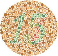
Colorblindness – Can you see the number in this image? 

This Distributome Activity illustrates an application of probability theory to study Colorblindness, typically a genetic disorder which results from an abnormality on the X chromosome. The condition is thus rarer in women since a woman would need to have the abnormality on both of her X chromosomes in order to be colorblind (whether a woman has the abnormality on one X chromosome is essentially independent of having it on the other).

Goals

The goal of this activity is to demonstrate an efficient protocol of estimating the probability that a randomly chosen individual may be colorblind.

Hands-on Activity

Suppose that \(p\) is the probability that a randomly selected ”man” is colorblind.

  • 100 men are selected at random. What is the distribution of \(X_m\) = the number of these men that are colorblind?
  • Answer

  • To estimate the probability that a randomly selected woman is colorblind, you might use the proportion of colorblind women in a sample of n women. What is the variance of this estimator?
  • Answer

  • Alternatively, to estimate the probability that a randomly selected woman is colorblind, you might use the square of the proportion of colorblind men in a sample of n men. Explain why this estimate makes sense. What is the variance of this estimator?

    See Hint

    Answer

  • For large samples, is it better to use a sample of men or a sample of women to estimate the probability that a randomly selected women is colorblind? Explain.
  • See Hint

    Answer

Alternate approach

You can also use the delta method to find the approximate variance for the estimator above.

Conclusions

In practice, it may difficult to obtain reliable parameter estimates when the event at hand is very rare (such as with colorblindness in women). The use of a valid probability model such as the relationship between the chance of colorblindness in men and the chance in women may improve these estimates.

Distributome Blog allows LaTeX Post Editing Using MathJax

The Distributome Blog now allows editing using MathJax-based math typography. For example:

  • Typing \\( \\int\_{\\pi}^{\\infty}{\\ln (x) dx} \\), replace the “\\” by “\” to render the formula in the blog page,
  • Would generate this: \( \int_{\pi}^{\infty}{\ln (x) dx} \)
For hidden fields you need to use the following alternatives as analogues of commonly used TeX/LaTeX syntax (as the JavaScript code behind the MathJax and the Hidden-answers plug-ins are incompatible):
  • For equal-sign “=”, use the \( \\equiv \) symbol (\(\equiv \))
  • For vertical bar “|”, use \( \\vert \) symbol (\(\vert \))
  • There may be other LaTeX/TeX alternative symbols that may need to be used for MathJax math typesetting in hidden fields!

Distributome Navigator: Ontology/Hierarchical Graph Display

We introduced a new Distributome.xml.pref file, which allows customization of the look-and-feel of the Distributome Navigator and Editor.

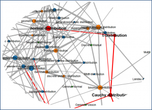
One example of this customization is the ability to display hierarchically the Ontology of the collection of distributions contain in the Distributome XML DB. That is we have a mechanism to render the nodes and edges as 3 levels: Top, Middle or All/Complete levels (affording to the pref file). The figure below illustrates this new hierarchical Distributome Navigator display.